Searching for Chinchilla Scaling in Tiny Arithmetic Transformers
Scaling Laws
Deep neural networks such as modern LLMs function as a kind of black box. We understand very little of what’s truly going on behind the trillions of floating point operations powering these tools. Lucky for us, there are ways to study these boxes without ever needing to open them. Among our limited arsenal lie scaling laws, which are empirical models that elucidate the relationship between our inputs (e.g. model size, training data, compute) and outputs (i.e. model capabilities)1.
Admittedly, “law” is a loaded term. These “laws” function much more like Moore’s law than Newton’s laws of nature; they are empirical observations, fitted on what we’ve actually built. So they are inherently conditioned on the realized path we took, as opposed to some fundamental unchanging truth about the universe on its own. This is important because there are often bottlenecks preventing us from achieving the degree of scaling modeled by these laws (just like how the chip industry had to resolve bottlenecks to “realize” Moore’s law)2. Once those bottlenecks are resolved, the laws then describe how certain input factors interact with one another, both directionally and numerically to influence the capabilities of our trained model.
Many interesting questions arise even as we operate within a scaling paradigm. While we can naively tune up all the input factors that are positively correlated with performance, the reality of resource constraints mean that we are often faced with tradeoffs. Let’s say we want to train some new model, and by divine benevolence we are granted 2x our original compute budget. Should we double our model size? Double our training data? Or a mix of both? These are the questions answered by Chinchilla’s law, the topic for this blogpost.
A simple model for models
To motivate this, suppose we want to derive some model for loss based on three key training parameters: model size (parameter count), training data size (measured in tokens), and compute budget (in floating point operations, or "FLOPs"):
Here, counts tokens processed during training, including repeated examples. We want to find the combination that produces the lowest training loss:
The first thing to note here is that conditional on a fixed model architecture, the three inputs are usually linked by some known function . This makes sense since our training FLOPs is dictated by the model architecture. We can approximate the transformer architecture as a massive stack of big matrix multiplications, which has a simple training compute formula3:
For example, Llama 2 7B (as in 7 billion params) was trained on 2 trillion tokens, so here FLOPs. Very handy formula! With this, we can take , and our original formula simplifies to .
Unfortunately, compute isn’t free4. With a fixed budget , our problem becomes simply
How do we solve this without knowing (or assuming) the functional form of ? Let’s hold this thought and return to our handy FLOPs approximation formula . Assume for some we already found the optimal , so we have . An interesting question we can ask is, if we were to scale to, say , what is the new optimal ? Comparing the old and new optimal values, we can define scale factors and . We know that by definition . Substituting, we get , which implies . Writing the scale factors as powers of two, and , this becomes
Stated plainly, this means that we need to distribute our compute scale factor 2 into a mix of model parameter count and training data size. The key question here is, how should we pick ?
Enter Chinchilla’s law
Chinchilla’s law helps us answer all these questions. Its answer to our last question is . This implies in our case. More broadly, it makes the observation that under fixed compute budget constraints, training data size should scale proportionally to model size. With this solution in mind, we can generalize the doubling example to an arbitrary scaling by a factor of : . Since this holds for any starting point we arrive at a power law
Something interesting happens when our exponent is 0.5. Consider the expression , which is the ratio of our training data size to model parameter count. By our handy formula we have . But since , this simply becomes
a constant independent of ! In other words, we have found that the optimal training data size to training parameter count ratio is a fixed constant independent of compute. This characteristic holds if and only if training data size scales proportionally to model size. And in Chinchilla’s case, this ratio was roughly 20 tokens per parameter. Quite magical!
To sum up, the contributions of Chinchilla’s law are three-fold:
- The rule of thumb that training data size should scale proportionally to model size
- The famous 20:1 training size to model parameter count ratio, known as Chinchilla optimality
- A fitted functional form for loss, with an irreducible term plus power-law penalties for finite model size and finite data:
Setting up a toy experiment for Chinchilla’s law
While we can certainly try to observe Chinchilla’s law by pre-training our own language model from scratch, it would also be interesting to see if the same empirical relationship holds beyond natural language modeling (and on a much, much smaller total compute budget). To investigate this, I took a simple 3-digit integer addition task and trained a collection of tiny transformer models, sizes ranging from 7k to 800k parameters, at varying compute budgets (hence training data sizes). Each example is a padded string like "123 + 456 = 579 ", tokenised character by character over a 13-symbol vocabulary (ten digits, +, =, and space), and the model is scored only on the digits (and padding) after the =.
How do we set up an experiment to observe this law? As we have already done the mathematical heavy lifting earlier, we know that it suffices to show . The constant token-to-parameter ratio follows naturally, though not necessarily Chinchilla’s particular ratio of 20:1. Taking log of both sides, this becomes
for a constant . One approach to verify this, is to choose a range of compute budget values , and for each , train models of varying sizes , and determine by taking the model that has the lowest loss. Then, we can take our pairs, take logs, and fit a linear regression to see if we recover 0.5 as the slope.
As always, there’s a handful of subtleties worth pinning down before committing to training runs. First, we have to ensure that our budgets are within a resource constraint regime, such that there still exists a real tradeoff between model size and training size. One can imagine some budget ceiling beyond which too many model vs training size pairs trivially solve the task. A task as simple as 3-digit addition would have quite a low ceiling; I measured this at around FLOPs, past which too many neighboring values have similarly low loss values, dampening our signal. At the lower end, I settled on FLOPs, where a tradeoff was still visible in the early experiments.
Second, as we train models of varying sizes especially in log scale, model performance becomes sensitive to hyperparameter choices, such as learning rate and batch size. The Chinchilla paper used larger peak learning rates for its smaller models than for its largest ones. This effect was indeed also present in my early training runs with a naive fixed peak learning rate of 3e-4, which overly penalized smaller models. After experimenting with various values with the goal of finding nice U-curves, I ended up using a small learning rate sweep of [3e-3, 1e-2, 3e-2], and selecting the learning rate with the lowest geometric-mean loss across the five seeds for each model size and budget5. As with the Chinchilla paper, I used a cosine learning rate schedule with warmup and decay6. For batch size, on the other hand, I kept it fixed at 128, as varying this did not seem to affect runs that much, so it made more sense to keep it a constant to isolate model size as the variable.
Unlike Chinchilla which measured training losses, my experiments chose based on held-out validation loss on 10% of the full dataset. The main reason here is that Chinchilla runs were sub 1 epoch, but for 3-digit additions there are only examples in total, and small models with large compute repeatedly revisit the same examples (up to about 17 dataset-equivalents in this sweep) to the extent that training loss stops being an unbiased estimator of loss on fresh data.
We repeat the same set of runs across 5 seeds. All runs were done on a TPU v5e-8 through Kaggle’s weekly 20hr free credits.
Results
Let’s first look at the “isoFLOP” curve for each compute budget and each seed. Each of these plots fixes a compute budget , and plots final test loss as a function of model parameter size . As we can see, each isoFLOP curve generally resembles a U-shape, which represents the tradeoff between allocating more compute to a larger model versus more training data.
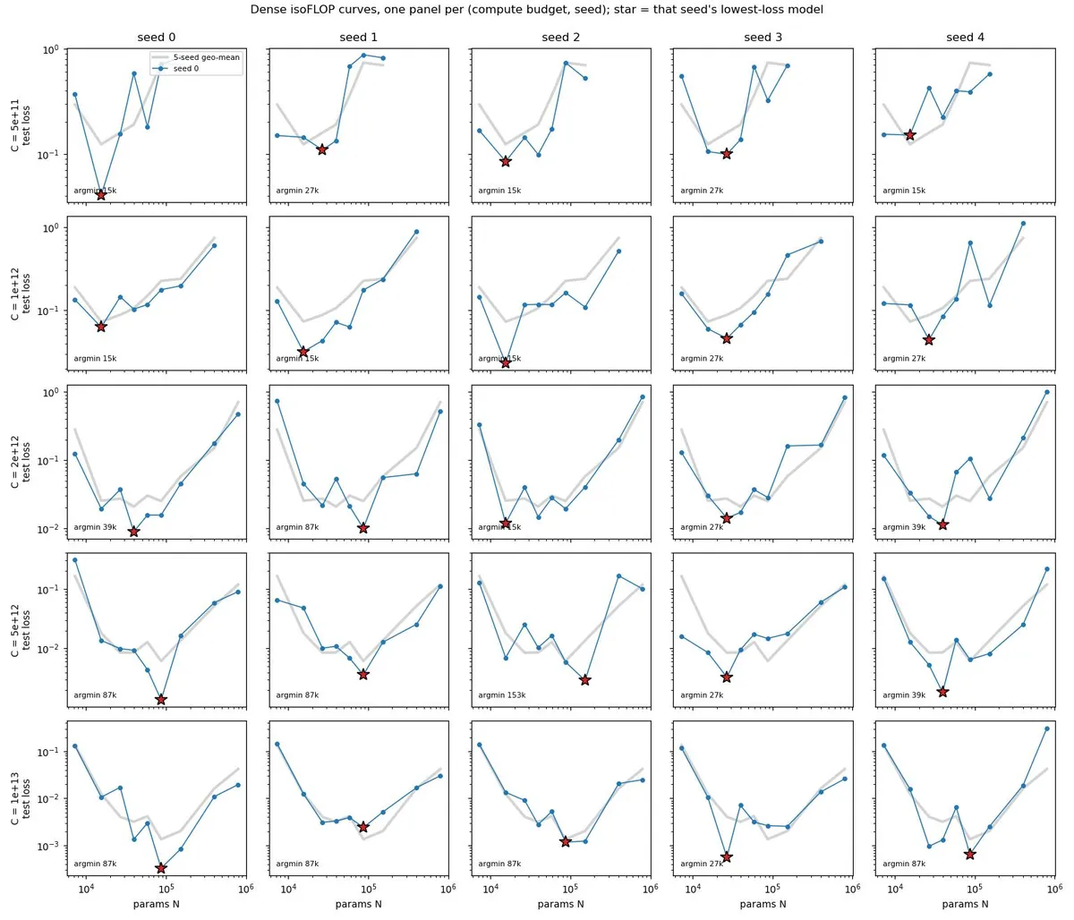
Eyeballing the graphs, we can already see that as we increase our compute budget (and move down the set of plots) the minimum test loss model parameter size generally increases. One thing that stands out here, though, is that there is a high degree of variability across the sweeps. For the same compute budget, not all seeds end up with the same optimal model size; there is also a lack of monotonicity on both sides of the flanks, though most curves generally follow a U-shape. At , for example, every model from 15k to 87k parameters lands within 25% of the best five-seed geometric-mean loss. That’s a small loss difference deciding between models nearly six times apart in size! A slight change in the losses can therefore produce a large jump in , even when the overall curve barely changes.
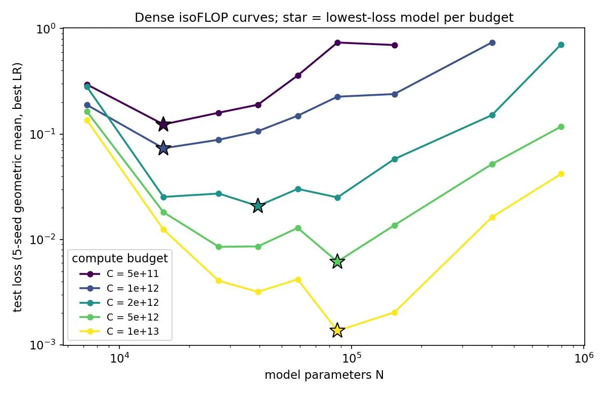
Averaging the five seeds cleans the curves up considerably, and the rightward drift of the minimum with compute becomes clear:
A parabola lets us use the flanks of the curve to help locate its bottom, instead of letting the lowest individual point decide everything. For each compute budget , we take the readings across all 5 seeds (45 points per budget), fit a 2-deg polynomial in and , and convert its vertex back into model size . The left panel below shows this at : the individual points at the bottom scatter by a factor of three across seeds, but the two flanks pin the parabola, and its vertex lands at 55k. We can then fit the pairs on a linear regression and find the slope, which was hypothesized to be 0.5 under Chinchilla’s law. We can also perform bootstrap resampling using our 5 seeds to find a 95% CI for the slope. The catch is that this stability comes partly from assuming a smooth quadratic curve. The bootstrap captures seed variability under that assumption. The right panel plots the regression, and we report our below:
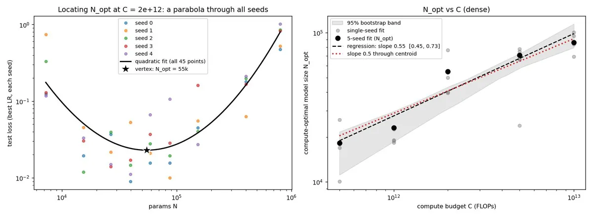
The regression gives, with a 95% bootstrap confidence interval over seeds,
and the fitted optima at each budget are:
| Compute budget (FLOPs) | N_opt |
|---|---|
| 5e11 | 18k |
| 1e12 | 23k |
| 2e12 | 55k |
| 5e12 | 71k |
| 1e13 | 86k |
So, did we find Chinchilla's law?
First, our fitted scaling exponent is compatible with Chinchilla’s ~0.5! Hurray!
The more interesting question to ask here is, did we have any reason to have a strong prior at all for the scaling exponent of 0.5, given that the trivial addition task at hand is fundamentally different from natural language modeling? Although our quadratic fits estimate some compatibility, our per-sweep and per-seed results, as the grid of isoFLOP curves above shows, seem quite noisy. Other than imperfections in resolving learning-rate sensitivity, perhaps one contributor is seed-sensitive learning transitions on this arithmetic task; we have been operating outside Chinchilla’s data regime. Unlike language modeling runs which have irreducible loss due to the inherent uncertainty in next-token prediction, our labels are deterministic and completely solvable. Different runs may learn digit alignment or carry handling at different times, producing large endpoint differences at a fixed budget. At high budgets, it becomes difficult to select a point estimate for , when a range of models produce similarly low test losses.
So within the budget range tested here, our fitted optima suggest that model parameter size should generally increase with compute. And the Chinchilla scaling exponent does lie within our confidence intervals. Whether that makes it Chinchilla's law or just a law-shaped coincidence on a toy problem, I'll leave to a reader with more digits.
Appendix: Mixture-of-Experts
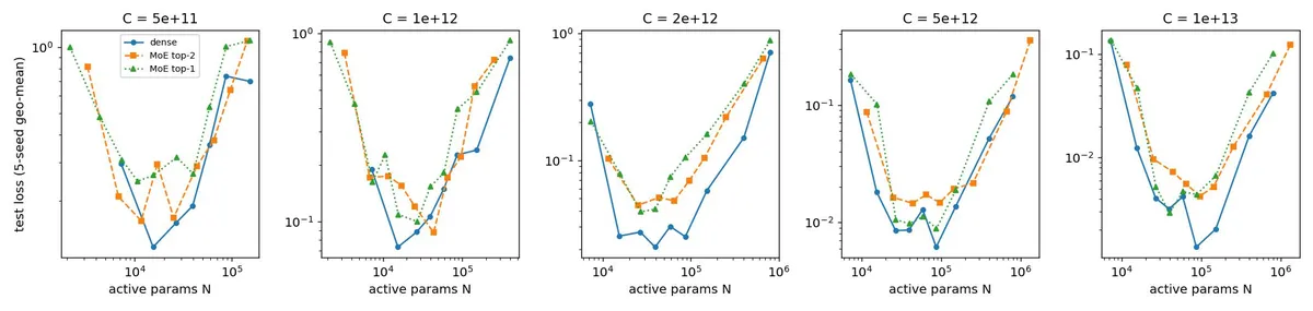
In addition to the dense model, I also ran the entire training loop on two Mixture-of-Experts (MoE) variants. Both had 4 experts (), with one having 1 activated expert and the other having 2 activated experts per MLP block (). For these sweeps we take as activated params, i.e. the parameters a token actually passes through, that is attention plus 1 or 2 of the activated experts. The fitted exponents come out similar. For , we get with a 95% CI of , and for , we get with a 95% CI of . The left plot below shows the best loss across all three model architectures per compute budget, and the right plot shows our log-log linear regression fits.
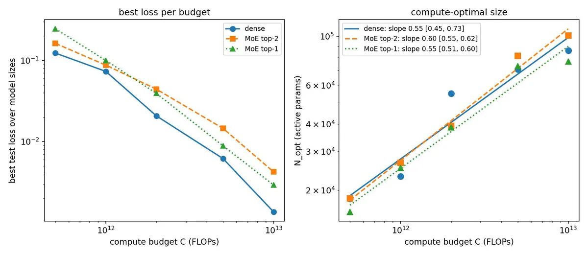
The main observation here is that at fixed compute, MoE does not reach the same loss as the dense model. The dense model reaches the lowest validation loss at all five budgets, with the gap widening at higher compute up to a factor of around 3, though with five seeds the smaller gaps are within noise. This makes sense, since the main purpose of MoE is to raise model capacity by storing more parameters than it uses per token, and this is a solution more relevant for regimes like language modeling whose loss is limited by model capacity. Three-digit addition is much simpler, so the added capacity goes unused, while the costs of routing remain. The cleanest evidence is the top-1 variant, which has the same active parameter count and the same number of training steps as the dense model, yet still ends up 1.5x to 2x worse. With each expert seeing only half or a quarter of the tokens but essentially trying to learn the same arithmetic patterns, the MoE models could be spreading learning signals too thin across their parameters.
Comparing between the two MoE variants, we see that the top-2 variant leads at the two smallest compute budgets, before falling behind at larger budgets, where top-1 leads by about 1.1x to 1.6x from 2e12 upward. One possible explanation for this is that since the top-2 model carries 1.7x the active parameters of the top-1 model (2x in MLP layers but same in attention), at each budget it gets fewer training steps, and under the higher budget regime training steps are the bigger bottleneck towards achieving better learning and generalization as opposed to model capacity. It would be interesting to see if we can generalize this training step vs capacity/sparsity scaling relationship for MoE architectures in the original language modelling context, and see how model sparsity scales with compute.
A great post that talks more about scaling laws: [https://lilianweng.github.io/posts/2026-06-24-scaling-laws/]↩
Another excellent read that discusses this in-depth: [https://www.beren.io/2026-08-23-Architecture-Research-as-Addressing-Constraints-to-Scaling/]↩
The first section of https://jax-ml.github.io/scaling-book/transformers/#counting-dots provides a good explanation for this formula↩
The natural question here again is, why even have compute budget constraints? Naively, one might think that a model should be trained to peak performance instead of subjecting it to compute constraints that would impose a performance ceiling. That’s actually a fair position, since most production models are apparently trained way beyond Chinchilla optimality. But given the ceaseless improvements in say architecture alone, one must subject each model generation/version to some fixed budget, or risk spending extra dollars squeezing a legacy model while competitors train on the latest SOTA. So clearly there is a separate, higher order resource allocation game here involving model cycles, inference costs, intelligence per training time/dollar spent etc. That game is way more complex, and overtraining beyond Chinchilla optimality is certainly a strategy for that game.↩
This differs from Chinchilla, which assigns each model size a single peak learning rate (from for its smallest models down to for its largest, per Appendix D.1 of the paper) and uses it across all token budgets. That assumes the best LR for a size doesn’t depend on budget. In my runs it drifts modestly, with larger models preferring a lower peak at the largest budgets, so I instead select the LR per (budget, size) cell from a fixed grid. The cost is three times as many runs and a coarse, 3x-spaced grid, so each reported loss is an upper bound on what a finely tuned LR would give.↩
This bit is actually crucial: the cosine decay should finish at the end of each run’s own training budget. If we evaluate a short run halfway through a much longer learning-rate schedule, we may underestimate how well it could have performed with a schedule tailored to its budget. Chinchilla identifies this as one important methodological difference from Kaplan et al.’s earlier scaling analysis, which suggested scaling model size faster than training tokens i.e. a model-size scaling exponent greater than 0.5.↩